Fractal Module Documentation by composer Warren Burt, PhD., www.warrenburt.com
Lorenz Pickover Martin Hopalong Hilbert Henon IFS6Dim
1dCA3 1dCA4 1dCA5 2dLife Duffing Algoart Mira
ArtWonk fractal modules are intended to be used as sources for both sound and graphics. Each tick produces an iteration of the fractal generator, and the outputs are available as floating point values, which can be scaled with the Math/Scale module.
Some programs give you a pre-composed set of mappings for Fractals into musical or visual parameters. With ArtWonk, since it's a construction kit for you to realize your own idea, just the raw fractals are given to you. It's up to the user to decide how the fractals will be used. However, each fractal has ranges for its parameters within which it gives you the best results. These are discussed in the notes below. Note that each output of the fractal produces an output that will be between varying number limits. In using them, you'll have to first observe the fractal in operation for a while, seeing what the limits of the output you want to use are, and then use either a Scale or a Bounds or a Mod or a Range module to put it within the limits you want. For example, to apply a fractal to a 640 x 480 pixel pallette, first determine the range of the output. If it goes negative, use an Add module to offset it so that the output of the Add is all positive. Then use a Scale to scale the output from whatever it is up to 640, 480 or whatever range you need. Many of the example files for the fractals do this kind of mapping of a fractal to a graphic. You'll find many helpful hints for mapping your fractal output to a useable range in them.
When used as a graphics source, the module should be put into a Loop macro. A loop count of 500-2000 will provide full screen graphics in a single tick cycle.
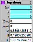
The Hopalong Fractal is a good one to start with. It's almost impossible to overload this equation. It will take just about any inputs you put into its A, B and C inputs - I've tried everything from -5000 to 5000 in the inputs, and a more or less interesting result almost always happens. The trick, though is in scaling the output to get a useful result. Set your A B and C parameters to the numbers you want to start with. Have the "reset" on the System module going into the "Reset" input on the Hopalong fractal module. Start your Clock (going into the "Chng" input on the Hopalong module) running. Put the X and Y outputs into a Peak module, and observe the results, seeing the highest value that appears in the Peaks. Let it run for a while, so you're sure you've gotten the highest value. This is usually somewhat less than three times the biggest value you have in any of the A, B or C inputs.
Put the output of the X and Y outputs into an Add module. Add a number a little bigger than the biggest value you got from the Peaks. Place the output of the Adders into Scale modules. Have the "From" input in the Scalars set to 2x the amount you added in the Adder modules. The "To" value in the Scalars should be the range you want your output to be over - for example 640 for video pixels, or 48 for pitches (for a 4 octave range). If you find you're getting values out of range, increase the values in the Adder and the "From" Values in the Scaler
| Largest value in A,B or C | Value to Add | "From" Value in Scaler |
| 5000 | 15000 | 30000 |
| 0.5 | 1.5 | 3 |
| 20 | 60 | 120 |
The problem with the Hopalong fractal is that the larger your iA, iB and iC values, the larger the output, and the smaller your iA, iB and IC values, the smaller the output. So when you scale your output for graphics or sound use, you have to take that into account. The demo patch, "ClassicHopalongGenerator.awp," shows that the ranges suggested for the input values, iA = +/-4; iB = +/-2; iC=+/-4 work well when 25 is added to the X and Y outputs and the Scale module From value is set to 50. The 5 presets - selected by the selection button - show some typical values. The values can be viewed in the Out1, Out2, and Out3 of the AMultiTap module. Note that the 4th and 5th use numbers outside the suggested ranges and things work just fine. This is to encourage you to experiment.
Outputs:
Iter: Iteration since last reset.
X: X point for current iteration.
Y: Y point for current iteration.
Inputs:
Chng: Any change calculates next iteration.
Reset: Reset and initialize.
iA-iC: Initialization constants. Try different values to change the fractal behaviour.
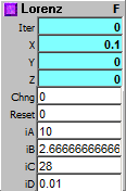
This is a fractal module that it's almost
impossible to overload. Ranges for the parameters are
at least
A -3200 to +3200
B -50 to + 50
C -600 to +600
D -250 to +250
However, if you go outside a very narrow range of values
near the middle of these ranges, most of
what you get, visually or sonically, will be pretty close to (un)equally
weighted noise.
To get the really fine grained complex structures that
the Pickover fractal is capable of,
one has to stick fairly close to the starting values.
A = 2
B = 0.5
C = -0.63
D = -2.5
If you leave the other three values alone, and change
just the one remaining value, the ranges that
fine-grained structures emerge within are approximately
A = 1 to 3 (or -1 to -3)
B = 0.1 to 1.5 (or -0.1 to 1.5)
C = -0.1 to -1.2 (or 0.1 to 1.2
D = -2.4 to -3 (or 2.4 to 3)
But be aware that within these ranges are "dead zones,"
where certain values will send the fractal
spiraling down into repeating one value, or looping through a few values.
Some of these "dead zones"
are
A around 1.6
C -1.40 to -1.55
D 0.5 to 2.3 and 3.7 to 4.4
Other ranges which produce either fine-grained structures, or which send the fractal spiraling down into repetition remain to be found.
The example file "Pickover Loop Tester.awp" will allow you to explore a wide range of values with this fractal rapidly. Each "frame" consists of 1000 interations of the fractal, so you can see how it builds up into structures rapidly. The example file "Pickover Explorer.awp" allows you to see the fractal drawn slowly, and listen to the individual values as they're drawn. In this realization, the Z output controls patch selection (use the internal GM synth for a cute version of this), so there's a different tone color every note.
Outputs:
Iter: Iteration since last reset.
X: X point for current iteration.
Y: Y point for current iteration.
Z: Z point for current iteration.
Inputs:
Chng: Any change calculates next iteration.
Reset: Reset and initialize.
iA-iD: Initialization constants. Try different values to change the fractal behaviour.
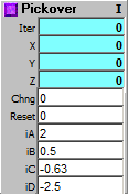
This is a fractal module that it's almost impossible to overload. Ranges
for the parameters are
at least
A -3200 to +3200
B -50 to + 50
C -600 to +600
D -250 to +250
However, if you go outside a very narrow range of values near the middle
of these ranges, most of
what you get, visually or sonically, will be pretty close to (un)equally
weighted noise.
To get the really fine grained complex structures that the Pickover
fractal is capable of,
one has to stick fairly close to the starting values.
A = 2
B = 0.5
C = -0.63
D = -2.5
If you leave the other three values alone, and change just the one
remaining value, the ranges that
fine-grained structures emerge within are approximately
A = 1 to 3 (or -1 to -3)
B = 0.1 to 1.5 (or -0.1 to 1.5)
C = -0.1 to -1.2 (or 0.1 to 1.2
D = -2.4 to -3 (or 2.4 to 3)
But be aware that within these ranges are "dead zones," where certain
values will send the fractal
spiraling down into repeating one value, or looping through a few values.
Some of these "dead zones"
are
A around 1.6
C -1.40 to -1.55
D 0.5 to 2.3 and 3.7 to 4.4
Other ranges which produce either fine-grained structures, or which send the fractal spiraling down into repetition remain to be found.
The example file "Pickover Loop Tester.awp" will allow you to explore a wide range of values with this fractal rapidly. Each "frame" consists of 1000 interations of the fractal, so you can see how it builds up into structures rapidly.
Outputs:
Iter: Iteration since last reset.
X: X point for current iteration.
Y: Y point for current iteration.
Z: Z point for current iteration.
Inputs:
Chng: Any change calculates next iteration.
Reset: Reset and initialize.
iA-iD: Initialization constants. Try different values to change the fractal behaviour.
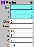
The Martin fractal is interesting because it just keeps growing. That is, over large numbers of iterations, the range of its outputs keeps increasing and increasing. These increases, however, usually don't happen for a while, then suddenly occur. For example, when mapping the fractal to a 640 x 480 graphic, with starting values of A=10; B= 11; C = 6; and D = 0.6, for the first 10,000 iterations, the diagram is fairly small, and stays in the middle of the picture, only covering about 1/3 of the picture area. After 10,000 iterations it suddenly expands to cover about 1/2 the picture. By 30,000 iterations, it has jumped again, now covering the entire picture. By 65,000 iterations it has expanded beyond the bounds of the picture plane. Input C seems to be the parameter that most controls this expansion, but its behaviour is not really linear. For example, with A = 10; B = 11; and D = 0.4; with C = 1, the picture stays very small, but does expand within tight limits. For C = 3 the image expands beyond the picture plane by 100,000 iterations, but for C = 4.3, the picture seems to stay at about 1/2 the picture size. Experimentation is the best way to explore this fractal.
The starting values of the module are A = 10; B = 11; C = 2; and D = 0.4. Leaving any 3 of these parameters at these starting values, and just varying one of them, the following ranges were found to work. Ranges beyond these might also work, but they haven't been explored.
The demo patch Martin Loop Tester with colors and sound.awp" allows you to see the fractal growing quickly. The sound is mapped in a bit more complex way - only every 100th point is used as data, and the data is mapped to pitches and durations of two different voices. "Martin Explorer.awp" allows you to directly change the iA to iD inputs while seeing the fractal drawn one point at a time.
Outputs:
Iter: Iteration since last reset.
X: X point for current iteration.
Y: Y point for current iteration.
Inputs:
Chng: Any change calculates next iteration.
Reset: Reset and initialize.
iA-iD: Initialization constants. Try different values to change the fractal behaviour.
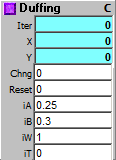
The Duffing Attractor lazily loops around a chaotic path, unpredictably traveling between two basins of attraction. The path can be changed by entering different values into the A and B inputs. The possible range of values for A is 0 to 1, and for B from -1 to +1, but not all combinations will work. Mostly, good values are found when A and B are both between 0 and 1, although some combinations will go into one basin of attraction, and stay there, such as the current Presets 1 and 12.
You will notice that the demo patch for this, "DuffingDemo.awp" is running fast - the System Main clock is set to 2, and the Clock running the Duffing Attractor is also set to 2. This is so that the attractor will be drawn in a reasonable length of time. This means that for the sound realization, the RanClock speed is set to 96, and still produces fairly fast notes. As is usual with these demo patches, X = pitch and Y = Velocity, and the addition of the RanClock means certain notes are "dropped," breaking up the musical line into phrases and rests. Additionally, you may want to put the Duffing Attractor into a Macro Loop for faster results.
Outputs:
Iter: Iterations since last reset.
X: X point for current iteration.
Y: Y point for current iteration.
Inputs:
Chng: Any change calculates next iteration.
Reset: Resets and initializes the function.
iA: Initial A value.
iB: Initial B value.
iW: Initial W value - best set to 1.
iT: Initial T value - best set to 0.
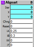
This is a unique fractal, found only in ArtWonk. It's loosely based on the equation for the Duffing Attractor, but not treated as a differential equation, and with limiting and a small amount of randomization thrown in. The nature of the attractor is best seen with "Line To" rather than painting with dots.
Hence in the demo patch, "AlgoArtFractalDemo.awp," in the Draw module, Actn is set to 1 rather than 2. To see the fractal with dots, just place a 2 in the Actn slot. The demo patch has 12 different Presets. These give some idea of the ranges to pick new values from. In general, values that work in the Duffing attractor will work here, but will give completely different results. The sound is a simple X=pitch, Y=velocity mapping, but with the RanFRClk set to 77% Rand, so rests are put into the resulting melodic line. I find the output of this attractor intriguing, especially when it's applied to pitch.
Outputs:
Iter: Iterations since last reset.
X: X point for current iteration
Y: Y point for current iteration
Inputs:
Chng: Any change calculates next iteration
Reset: Resets and initializes the function
iA: Initial A value
iB: Initial B value
iW: Initial W value - best set to 1
iT: Initial T value - best set to 0
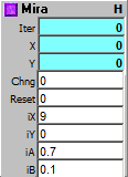
The Mira Fractal generates lots of interesting patterns, all centered and symmetrical. The 12 Presets in the demo patch "MiraDemo.awp" only scratch the surface of what this fractal can do. The patterns need lots of time to develop. For many settings, after several thousand iterations, a new part of the pattern emerges. Further, this fractal needs high resolution to really see the detail it makes. A resolution of at least 640x480 is recommended.
The demo patch is running fast. System Main is at 3 and the Clock is at 3. This is to show the development of the fractal in a reasonable amount of time. To see quicker development, use the fractal in a Macro Loop.
The values in the Presets were derived by altering one parameter a little at a time, as you'll see if you step through them, observing the values on the Number Grid below the presets. Explore to see how far you can push this.
The sound in the demo patch simply uses a RanFRClk, set to happen 75% of the time, with X = pitch and Y=velocity. The durations in the RanFRClk are larger than expected because the Main clock in the System module is set to a very low 3, to push the drawing faster. There are more interesting ways to realize sound, but this one gives an indication of some possibilities of the fractal.
Outputs:
Iter: Iterations since last reset.
X: X point for current iteration
Y: Y point for current iteration
Inputs:
Chng: Any change calculates next iteration
Reset: Resets and initializes the function
iX: Initial X value
iY: Initial Y value
iA: Initial A value
iB: Initial B value
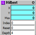
The Hilbert, or Space-Filling curve, is different than the other fractals. It is not triggered along with a strobe, or a change, but with an address. Inside the Hilbert fractal is an array of points. You select those points with the address that you put into the Index input. If you put a simple linear counter, counting by 1 into the index, and draw a line from one point to the next, you get the classic Hilbert "curve" - a succession of straight lines at right angles to each other. The Depth input selects how many points the curve has, from 3 with a setting of 1, through 255 with a setting of 4, up to 65535 with a setting of 8. The depth can only change however, when a strobe is received at the Reset input, which also sends the Index count back to 0.
Where the Hilbert curve gets really interesting, however, is when a non-linear set of values is put into the Index. For example, have a counter Incrementing by 17, with a top value of 10000. Put the output of the counter through an IMod set to 253, with the Depth of the Hilbert counter set to 4. By drawing lines between each new point, wonderfully erratic drawings, which eventually coalesce to a possible symmetry are made. Another use is to use the Hilbert to specify the point at which images are placed in a screen. Interesting juxtapositions of images can be made in this way. For music, using ideas such as the above, and scaling the output appropriately can produce some interesting "found-object" sequences.
The demo patch "FrHilbert.awp" shows the basic Hilbert function. The demo patch "HilbertExtendedVideoDemo.awp" shows an extended and highly processed version of the function. Using the values given in the above paragraph, but with Depth set to 5, the output is graphed with LineTo, and then delayed versions of the outputs control Color and Mosaic Amt, and the graphic is also processed with Erode. For sound, X controls the pitch of one voice, and Y controls the pitch of another. The clocks are RanClocks, set to only play 66% of the time, and the two voices are in a rhythmic ratio of 6:7. This produces something a bit more complex than just the simple Hilbert curve.
With this fractal there are no limits to exceed, and the outputs of X and Y are always from 0 to 1, so it's an ideal module to experiment with without worrying about things going out of range
Outputs:
X: X point for current iteration.
Y: Y point for current iteration.
Max: Maximum points in curve.
Inputs:
Index: Address index (0-Max) of point..
Reset: Reset and initialize.
Depth:Recursive depth (1-8), larger values for smaller curves, so you'll have to Scale the outputs differently to get the same size diagram for different Depths.
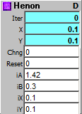
The Henon attractor is, again, one of the oldest fractals. It's also VERY sensitive to small changes in its inputs. This module allows you to play around with all 4 variables in the equation. Again, iA and iB are VERY sensitive - they can only be varied within a narrow range. I've found iA can work from 1.42 down to about 1.2, iB between .291 and .304. The classic values for them are iA = 1.42; iB = .3.
X & Y use values between 0 and 1. Not all values between these ranges will work, however. For example, these are X, Y pairs that work: {.3, .4} {.8, .2} but these are X, Y pairs that DON'T work, and send the equation off into infinity: {.6, .9} {.5, .8}.The selection button has three sets of values which work, and which shape the attractor in slightly different ways.
For more variation on this fractal, adjusting the "Add" and "Scaling" values for the attractor output will allow "zooming in" to the graphic for a look at more detail of the fractal's structure. In fact, in research settings, most of the interest in the Henon attractor is in just this kind of "zooming in," allowing one to observe the similarity of the zoomed in structure with the larger structure.
In the example patch "Classic Henon Demo.awp" three different presets are given. Sound uses X for Pitch and Y for Velocity. Of course, there are more interesting sound mappings than this, although this simplistic mapping allows aspects of the structure of the fractal to be heard readily. The pitch map "Bebop2" gives the resulting music a certain bounce and piquancy.
Outputs:
Iter: Iteration.
X: X point for current iteration.
Y: Y point for current iteration.
Inputs:
Chng: Any change calculates next iteration.
Reset: Reset and initialize.
iA: Initial A value.
iB: Initial B value.
iX:Initial X value.
iY:Initial Y value.
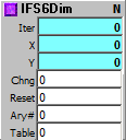
The 6 dimensional IFS (Iterated Function Systems) fractal is a very powerful generator of a wide range of images. Tiny changes in the values can produced radically different images. Two good programs that allow you to gain familiarity with the IFS system are both old DOS programs, now available for free download: "James Gleick's Chaos" and "Fractint." These are available on the web:
Chaos: http://www.cs.sjsu.edu/~rucker/chaos.htm;
Fractint: http://spanky.triumf.ca/www/fractint/fractint.html.
Both of these programs should run on most versions of Windows.
The key to the IFS module is that it needs an array of values, arranged in a 7 x 4 matrix. There are 6 values for the variables, and one probability value for each line. The easiest way to enter values is to type the values your interested into a text editor, save the file, then use DataBin to convert the typed values to an ArtWonk array. Then within an Array Module, you can load the .awa Array file, and plug the number of the Array into the Ary# input on the IFS6Dim module. Multiple sets of 28 values can be loaded into an array. The Table input on the IFS6Dim module multiplies the input integer by 28 to give the starting point for the next image.
This is best shown in the demo patch "6D IFS Array Loader Test.awp," which shows 8 oldies by goodies, tried and true IFS diagrams with values taken from the old DOS programs Fractint and James Gleick's Chaos. The actual values for these are shown in the module "IFS VALUES" just below ArySameNum in the upper left. Click on the IFS VALUES module to open up a "Text Notes" window which has all the numerical values for these fractals.
The demo patch "6D IFS Slider Array With Sound.awp" adds an array of sliders controlling the IFS 6Dim module. The values are making a shape I found pleasant. You can experiment with changing the values to see how each affects the overall diagram. MAKE SURE the Prob values are only set to positive values. The changed values will only affect the diagram on restarting of the program with the play button. In this patch, the FitScale module is used to put the pitches into the "Arabic" scale. This is in homage to Al Khwarizmi (780-850), Iraqi-Persian mathematician who invented the idea of following a series of steps to gain a mathematical goal, thus starting off this whole algorithmic thing.
The final demo patch is "6D IFS Sierpinsky with sound.awp." Here, an array of sliders controlling the IFS 6Dim module make the classic Sierpinsky Triangle. You can experiment with changing the values to see how each affects the overall diagram. MAKE SURE the Prob values are only set to positive values. The changed values will only affect the diagram on restarting of the program with the play button. The FitScale module is used to put the pitches into the "Bebop 1" scale. I'm sure Thelonious Monk, Charlie Parker or Dizzy Gillespie would have been fascinated by the IFS system.
Outputs:
Iter: Iteration.
X: X point for current iteration.
Y: Y point for current iteration.
Inputs:
Chng: Any change calculates next iteration.
Reset: Reset and initialize.
Ary#: Array number for 6 dimension initialization (4 sets of a-f & probability = 28 values per init table).
Table: Init table (multiplied by 28 to give table # offset in array).

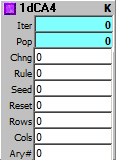

1 dimensional Cellular Automata with 3, 4 and 5 cell neighborhood
The 1D Cellular Automata systems (given here in 3 flavors) allow you to explore the world of Cellular Automata, one of the first areas in which the idea of "Artificial Life" was explored. In the demo patch "CellularAutomataDemo.awp," the top horizontal line of the LEDGrid is a set of cells. These are compared with their neighbors to determine if a given cell is a 1 or a 0 in the next generation. Each subsequent generation moves down the grid. The output of the CA module is an Array of values, shown with the LEDGrid. For sound output, the output of the array is read with an AMultiTap, 8 bits at a time, and converted to a number with Bits2Num. So the leftmost 8 bits of this CA make one number, and the rightmost 8 bits make a different number. These numbers are scaled and applied to pitch and loudness of two Midi voices. There are many other ways to get values off the Array, but this shows one possibility.
The slider in the demo patch allows you to pick different rules while the patch is playing. But if you generate a row with no values in it, you'll have to restart the patch to reseed the grid with a new starting value. Some of the rules will generate simple repeating patterns, while others will generate cycles of greater interest.
For one of the best summaries of how Cellular Automata work, what rule sets are fruitful, etc. go to Dave Burraston's website, where you'll be able to download a number of his research papers, including his 2006 PhD dissertation on Cellular Automata and music. http://www.noyzelab.com/research/research.htm
Outputs:
Iter: Iteration.
Pop: Population of live cells per iteration.
Inputs:
Chng: Any change calculates next iteration.
Rule: CA Rule 0-127.
Seed: Seed on Reset: integer to set bits, 0.01 to 0.99 for rand density.
Reset: Strobe to clear and seed, strobe <0 to also clear history.
Rows: Rows is history, each iteration bumps top row down.
Cols: Columns is Number of cells to process.
Ary#: Array number to use for 1dCA and its history.
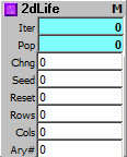
Conway's game of Life 2d Cellular Automata.
Conway's Game of Life is a classic. It's been written about in many books, and many people have explored it in depth. A free program that explores it, and many variants of it is Mirek's Cellebration. http://psoup.math.wisc.edu/mcell/ ArtWonk's 2dLife implements the most common Life rule, and lets you explore it easily.
In the demo patch, "GameOfLifeDemo.awp," a counter advances horizontally through the array showing the current generation of Life. Whenever the counter reaches the end of the row, a new generation of Life results. The top 4 horizontal rows are read here like a drum machine grid. Blue = on, Orange = off. They are controlling four voices which are playing one each of the notes of a Major Seventh chord. There are many other ways of using the Life information, but this patch will get you started.
The demo patch "LifeDemo02.awp" shows how the integer reseed works. Any integer up to 32 bits (ie, from -2,147,483,648 to +2,147,483,647) will seed the first 32 cells of the Life Array. After that the pattern will be fully or partially repeated. How the pattern appears and is repeated, and how it's operated upon by the Life2D module depends on the size of the Life Array, specified in Rows and Columns. In the "LifeDemo02.awp" patch, a grid of 8x4 cells is set up for input into the 32 bits of the array. This is realized as an 8x8 and a 9x9 Life Grid. As you will see in the patch, these two grid sizes produce very different results. Inputting patterns in this way, in conjunction with any of the standard books or articles on Conway's Game of Life, will allow you to explore the many kinds of patterns, such as "glider guns," that Life produces.
Outputs:
Iter: Iteration.
Pop: Population of live cells per iteration.
Inputs:
Chng: Any change calculates next iteration.
Seed: Seed on Reset: Any integer from -2,147,483,648 to +2,147,483,647 to set bits 0-31; 0.01 to 0.99 for random density.
Reset: Strobe to clear and seed.
Rows: Rows of cells in game board.
Cols: Columns of cells in game board.
Ary#: Array number to use for Life 2dCA results. Newly born cells are set to 2, other live cells are set to 1.
ArtWonk is Copyright © 2003-2014 by John Dunn and Algorithmic Arts. All Rights Reserved.